usbtrio.blogg.se - august 2022

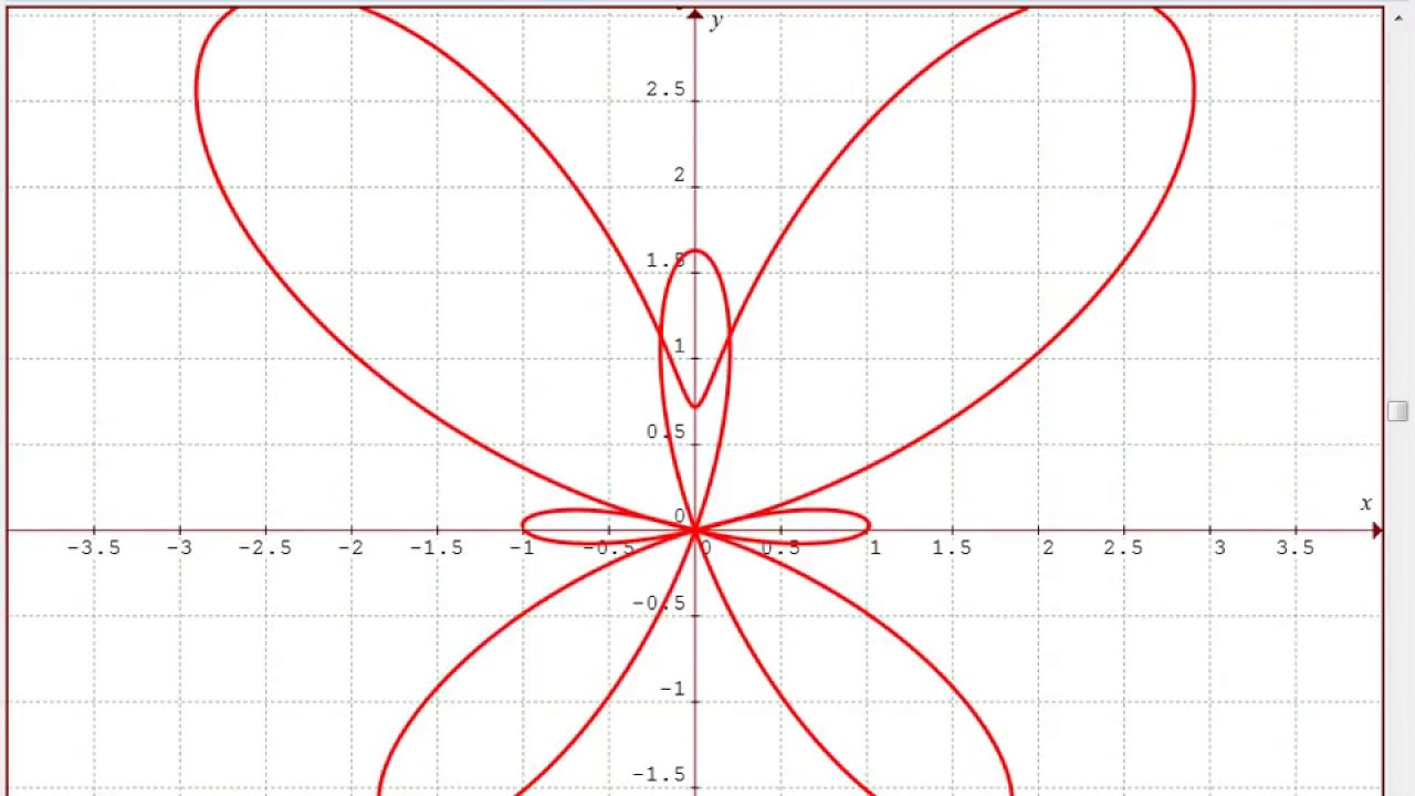
The Point tables show values at an interval and precision that you control, so you can get detailed numerical results or practice sketching curves yourself. Pause and Point tables options let you see the coordinates of points on your graphs.Easy to use controls, including a toolbar, right-click popup menus, the status bar, which displays relevant information and help messages, and the Redraw Queue combobox, which lets you select any equation in memory to graph, delete, or edit to form a new equation.Data plotting and curve fitting support make it easy to highlight points on a curve or enter experimental data sets and find the equation of best fit.

Most graphs appear instantly on modern machines. Cartesian inequalities are supported as well. You can choose between six styles of graphing: regular Cartesian, polar, parametric, and slope-field and initial-value approximations for up to fourth-order ODEs (and fourth-order linear systems as well), all detected automatically based on which variables you use in your equation. Forget about isolating variables before graphing! Graphmatica will isolate the dependent variable for you, if possible, and even graph many relations that can only be specified as implicit functions. You can use implied multiplication, a complete library of math functions (including trig), and even leave out those annoying parentheses in appropriate places.

Advanced equation parser follows mathematical rules-not the computer's.

You can save your work for use in a later session or with any text editor. Graphmatica remembers up to the last 999 equations you typed in or loaded from a file. Remember, here is todays assignment and there is tutoring after school until ten to five with Mr. Therefore sin is "+" and because tangent is a negative value, it cannot be quadrant one because X and Y are both positive. This is a similar question to the one above where we discovered that Theta was in quadrant II because Sin > 0. Here we were just applying signs to values in terms of quadrants and the location of the coordinates. This picture is continued from the picture above. We also talked about calculating cosecant, secant, and cotangent. While we were reviewing the unit circle we found it handy to think in proportional triangles to find the values for sin, cos, tan etc. The class was also introduced to more radian measure and learning to think about what quadrants they apply to. He got us thinking in terms of sinΘ - referring to Y, cosΘ - referring to X, and tanΘ - X/Y. Maksymchuk explained some more about the Unit Circle.

The image to the side was also handed out. Then at the end of class we were assigned questions 1-15 on exercise 5 and 1-16 on exercise 6. Then the class was then introduced /reminded of definitions and formulas for them which are on the slides below. Also the mostly vertical lines are the remaining function tan and cot with tan being the lines bending to the right going from bottom to top and cot being a mirror image of tan. The parabola's are formed by the csc and sec graph's and they touch the greatest value of there corresponding function i.e sec touches sin's greatest values. The image below was handed out in class and has all he functions on the same graph. Next was the actual graphing of the functions on graphmatica and ow it can relate to the unit circle i.e Y=sin(x) is greatest at π/2 on the graph and is positive up until π, which is equivalent to quadrants I and II on the unit circle. Then was a bit Review with the definitions of Domain( the values that x can be) and Range ( the values that y can be) The definition of Asymptote given on the slide below is also very important to know Sec and cot are done like csc meaning sec is (y= 1/cos theta) and cot is (y= 1/tan theta). Next came Reference Curves with a " how-to" lesson in putting the six trig functions into a calculator or other technological device as shown by the image below.